Elasticsearch APM: What Traces Show and Where They Stop
Elasticsearch APM: What Traces Show and Where They Stop
Elastic APM is a trace pipeline with a UI bolted on top, and that framing answers most confusion about it upfront. The moment you treat it as a dashboard, you start asking it questions it was never built to answer. The moment you treat it as a pipeline, you start asking the right one: how long did this specific Elasticsearch call take, on behalf of which user request, and where did that time actually go?
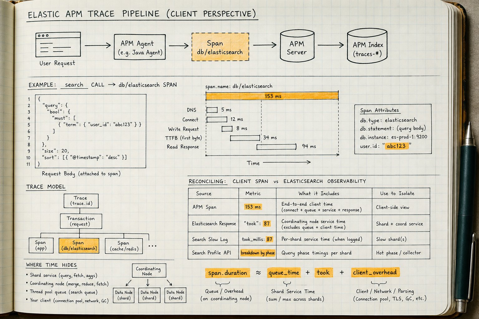
I have been paged for a slow checkout page that turned out to be a Postgres lock wait, and I have been paged for a slow checkout page that turned out to be Elasticsearch fanning a _search request across four hundred shards. The pager sounds the same either way. What differs is the muscle memory you need to diagnose it — and if you have spent years living in pg_stat_statements and auto_explain, Elastic APM will feel familiar and foreign at once. What does not transfer for free is knowing where client-side measurement ends and server-side measurement begins. That seam is the whole article.
What Elasticsearch APM actually monitors (and what it doesn’t)
Four moving parts make up elastic apm application performance monitoring:
- An agent inside your application process. A classic Elastic APM agent (Java, Python, Node.js, Go, .NET, Ruby) or, increasingly, an Elastic Distribution of OpenTelemetry (EDOT) SDK. It hooks libraries, times things, buffers events.
- APM Server. Receives events over HTTP, validates them, writes them to Elasticsearch. In Fleet-managed deployments this is the APM integration running under Elastic Agent rather than a standalone binary — same job either way.
- Elasticsearch as the store. Trace data lands in data streams named
traces-apm-*,metrics-apm.*andlogs-apm.*. - Kibana as the reader. Waterfalls, service maps, latency distributions.
Here’s the misconception, stated plainly so it dissolves: Elastic APM does not monitor your Elasticsearch cluster. It monitors applications. If one of those applications happens to be a Java service calling _search, you get visibility into that call from the caller’s point of view. The cluster itself is monitored by a different toolset entirely (Stack Monitoring, cluster stats, node stats).
So here is what APM will never tell you:
- Which shard was slow, or how many shards the request touched.
- Segment count, merge pressure, or how long a force-merge has been dragging.
- JVM heap pressure, GC pause duration, or circuit breaker trips on a data node.
- Whether the query got a hit in the request cache or the query cache.
- Whether your query was rewritten into something expensive.
APM gives you a wall-clock number attached to a named user request. Everything above lives on the other side of the socket, and you get it from cluster-side tools: _nodes/stats, _cat APIs, the slow log, the Profile API.
Elastic APM spans and transactions: the data model
The model is a tree, and the vocabulary is worth getting exactly right, because you will eventually query the raw documents.
- A transaction is one top-level unit of work: an inbound HTTP request, a consumer poll, a cron job tick.
- A span is one child operation inside that transaction, typed by
type/subtype/action. - Spans nest inside other spans through parent IDs.
- A trace is the whole tree, potentially spanning multiple services, stitched together by a shared
trace.id.
Cross-service stitching happens over the W3C Trace Context traceparent header. Elastic agents historically also emitted a vendor-specific elastic-apm-traceparent header for backwards compatibility, still visible on the wire in older fleets.
Every event carries four fields worth memorising:
| Field | Meaning |
|---|---|
trace.id |
The whole tree. Stable across services. |
transaction.id |
The top-level unit this event belongs to. |
span.id |
This span’s own identifier. |
parent.id |
The span or transaction directly above it. |
These fields aren’t UI decoration. They let the same trace get reassembled across service boundaries when your checkout service calls your inventory service, and they let you query raw documents in Kibana’s Discover view or via the Elasticsearch REST API directly — bypassing the APM UI when it isn’t showing you what you need.
Here’s a trimmed, annotated pair, transaction first:
{
  "@timestamp": "2026-07-29T14:02:11.481Z",
  "processor": { "event": "transaction" },
  "trace":       { "id": "4bf92f3577b34da6a3ce929d0e0e4736" },
  "transaction": {
    "id": "00f067aa0ba902b7",
    "name": "POST /checkout",
    "type": "request",
    "duration": { "us": 912480 },      // 912 ms end to end
    "sampled": true
  },
  "service": { "name": "checkout-api", "environment": "prod" }
}
And one of its Elasticsearch children:
{
  "@timestamp": "2026-07-29T14:02:11.702Z",
  "processor": { "event": "span" },
  "trace":       { "id": "4bf92f3577b34da6a3ce929d0e0e4736" },
  "transaction": { "id": "00f067aa0ba902b7" },
  "parent":      { "id": "00f067aa0ba902b7" },   // parented on the transaction
  "span": {
    "id": "b7ad6b7169203331",
    "name": "Elasticsearch: POST /products/_search",
    "type": "db",                                 // the pair that matters
    "subtype": "elasticsearch",
    "action": "request",
    "duration": { "us": 812340 },                 // 812 ms measured in-process
    "db": {
      "statement": "{\"query\":{\"bool\":{\"filter\":[{\"terms\":{\"sku\":[\"...\"]}}],\"must\":[{\"match\":{\"title\":\"wireless keyboard\"}}]}},\"size\":50,\"aggs\":{\"by_brand\":{\"terms\":{\"field\":\"brand\",\"size\":200}}}}"
    },
    "destination": { "address": "es-coord-3.internal", "port": 9200 }
  }
}
span.type: db plus span.subtype: elasticsearch is the signature you filter on. Learn it — the Kibana UI abstracts it away, and the raw query does not.
How the agent measures your Elasticsearch calls
The mechanism is unglamorous and worth understanding precisely, because it defines the measurement boundary.
The agent auto-instruments the official Elasticsearch client: the Java RestClient/ElasticsearchClient, elasticsearch-py, @elastic/elasticsearch, and so on. It wraps the client call site, starts a span immediately before the HTTP call is dispatched, and ends it after the response has been read. Duration is wall clock, measured entirely inside your process. It captures method, path, response status, target host and port.
For search-style endpoints it also captures the request body into span.db.statement. On the Java agent this is governed by elasticsearch_capture_body_urls, whose default allowlist covers search-shaped endpoints (*_search, *_msearch, *_count, *_search/template) rather than every request. It does not capture bodies for arbitrary index or update calls by default. That’s a good default, for two reasons:
- PII. A
_searchbody frequently contains user input verbatim — exact query terms, a geo bounding box tied to a delivery address, a raw customer identifier used as a filter clause. That value is now sitting in an Elasticsearch data stream with whatever retention your ILM policy allows, which is rarely the same retention policy as your application logs. - Size. A bulk index body can be megabytes. Capturing it would be self-defeating.
If you’ve moved to OTLP ingest or an Elastic Distribution of OpenTelemetry, the concepts are identical and the attribute names shift to OpenTelemetry semantic conventions, where db.system carries the value elasticsearch — the direct analogue of Elastic’s db/elasticsearch pair. APM Server ingests OTLP natively, so you’re looking at the same tree either way, and everything in this article applies to both.
Reading a waterfall: a real N+1 hiding in Elasticsearch query performance
Real case, lightly anonymised. POST /checkout at p95 of 912 ms. The team’s ticket said “Elasticsearch is slow.”
The waterfall said something more specific. Under the transaction:
POST /checkout ......................................... 912 ms
├─ db.postgresql SELECT cart ............................. 4 ms
├─ db.elasticsearch POST /products/_search .............. 812 ms
│   (span compression: 37 similar spans)
└─ external.http POST /payments .......................... 71 ms
One line, 812 ms. Except it wasn’t one call. It was 37 sequential _search calls averaging 18 ms each, one per cart line item, collapsed by span compression into a single row.
This is the single most important UI caveat in Elastic APM: agents compress runs of short, similar, sibling spans into one representative span carrying a count, so the waterfall doesn’t render forty nearly-identical rows. It exists so a 500-span N+1 doesn’t blow your event budget, and it’s the right trade. But if you skim the waterfall and read “one Elasticsearch call, 812 ms,” you’ll go hunting for a slow query that doesn’t exist, or badly undercount calls if you’re chasing a rate-limit or connection-pool-exhaustion issue. Expand the compressed span, or query the underlying documents directly. Read the count.
APM found the shape of the problem in about ninety seconds — an N+1 pattern hiding behind a plausible-looking single-digit-millisecond-per-call latency. It did not find the cause, and it couldn’t have: each individual query was fine. The fix was code, not cluster tuning — an _msearch and, later, a single terms query.
Which brings us to the part APM alone cannot do.
The gap that matters: span duration vs took
Every Elasticsearch search response carries took, in milliseconds. took is measured on the coordinating node: it covers the time the search spent inside Elasticsearch. It does not include request serialisation in your client, network transit in either direction, or time your request spent waiting for a free connection in the client’s connection pool.
Your APM span is measured inside your application process, from just before dispatch to just after the response is read.
Subtract them:
span.duration - took = client serialisation
                     + connection-pool wait
                     + network transit (both ways)
                     + response deserialisation
That gap is not noise. It’s a directly usable measurement of everything outside Elasticsearch, and almost nobody computes it.
Worked example from the checkout case, taking one uncompressed span:
span.duration.us = 18_400        ->  18.4 ms
took             = 3             ->   3.0 ms
difference       =                   15.4 ms  (84% of the call)
Fifteen milliseconds of overhead on a 3 ms query, thirty-seven times over. The cluster was innocent. The client’s connection pool was sized at 10 against a service running 64 request-handling threads, and the aggregation response was 340 KB of JSON being deserialised into objects for a page that displayed twelve fields. Other times the suspects differ: TLS handshake on a cold connection, DNS resolution against a load balancer, or genuine network latency if the coordinating node sits in a different availability zone than your app pod. I’ve seen all of these be the actual answer in different incidents, and the fix in each case was entirely on the client side.
To use this routinely, log took from the response as a labelled field on the span:
// Java, classic agent
SearchResponse<Product> resp = client.search(req, Product.class);
Span span = ElasticApm.currentSpan();
span.setLabel("es_took_ms", resp.took());
span.setLabel("es_shards_total", resp.shards().total().intValue());
Now you can chart span.duration.us / 1000 - labels.es_took_ms and alert on it.
The decision table I keep in a runbook:
| Span duration | took |
Per-shard query time | Read it as |
|---|---|---|---|
| Large | Small | n/a | Client-side: connection pool wait, serialisation, GC in your app, or network |
| Large | Large | Small | Coordination, fan-out across many shards, thread pool queueing, or fetch phase |
| Large | Large | Large | Genuine shard work: expensive query, cold cache, heavy aggregation |
| Small | Small | Small | Volume, not latency. Count the spans. Look for the N+1 |
I use this table before I open a single cluster-side tool. It tells me which of the next sections is worth my time.
Elasticsearch slow log vs APM: crossing into cluster-side tools
Once the table points you server-side, you have three tools, each with a specific blind spot.
Search slow log
Configured per index with dynamic settings, with separate thresholds for the query phase and the fetch phase:
PUT /products/_settings
{
  "index.search.slowlog.threshold.query.warn": "1s",
  "index.search.slowlog.threshold.query.info": "500ms",
  "index.search.slowlog.threshold.query.debug": "200ms",
  "index.search.slowlog.threshold.fetch.warn": "500ms",
  "index.search.slowlog.threshold.fetch.info": "200ms"
}
The blind spot, and the crux of elasticsearch slow log vs APM: thresholds are evaluated at the shard level, not for the request as a whole. A search that fans out across 400 shards and takes 900 ms overall can spend 4 ms — or even 12 ms — on every single shard, sail under every threshold you’ve set, and never trip a thing. The slow log will stay silent about a request that was, from the outside, genuinely slow. This is exactly the “large took, small per-shard time” row in the decision table above, and it’s the row where the slow log will actively mislead you if you don’t already know its scope. This is the most common reason someone tells me “the slow log is empty, so Elasticsearch is fine” when it isn’t. Set these thresholds before you need them; a dynamic settings change during an incident is one more variable.
Thread pool counters
When took is high but per-shard query time is low, check whether requests were sitting in a queue:
GET _cat/thread_pool/search?v&h=node_name,name,active,queue,rejected,completedor, with more detail:
GET _nodes/stats/thread_poolNon-zero rejected is unambiguous. A persistently non-zero queue on a subset of nodes tells you the coordinating node is spending time waiting for a worker rather than doing shard work — consistent with fan-out or concurrency pressure rather than any single slow shard.
Search Profile API
For per-shard, per-query-component timing, the Elasticsearch Search Profile API is the closest thing to EXPLAIN ANALYZE:
GET /products/_search
{
  "profile": true,
  "query": { "bool": { "must": [ { "match": { "title": "wireless keyboard" } } ],
                       "filter": [ { "terms": { "sku": ["A1","B2"] } } ] } },
  "aggs": { "by_brand": { "terms": { "field": "brand", "size": 200 } } }
}
You get a breakdown per shard, per query component, plus aggregation timings. Elastic warns explicitly that profiling adds significant overhead and shouldn’t be enabled by default in production. Treat it like EXPLAIN ANALYZE on a busy primary: run it deliberately, on a replica if you can, against a reproduction of the real query, get your answer, and turn it back off. The output is also genuinely enormous — budget screen space.
The Profile API’s own blind spots: no network time, and the fetch phase isn’t broken down in the same shape as the query phase — don’t expect a single unified number the way EXPLAIN ANALYZE gives you. If your took is large and the profile output sums to a fraction of it, look at fetch, coordination, and reduce.
Correlating logs and distributed traces without grep
Elastic APM agents inject trace.id, transaction.id and span.id into the application’s logging context (MDC in Java, structlog processors or the logging filter in Python, and equivalents elsewhere). Once your log lines carry those fields, joining application logs to a trace in Kibana becomes a filter, not a grep — no aligning two clocks by eye and hoping.
The pattern I recommend on day one:
- Turn on log correlation in the agent config and confirm
trace.idis present in a real log line before you go further. - On every Elasticsearch span, set labels for
took, total shards, and skipped shards. - Log the Elasticsearch request path and the index pattern at debug level with the trace context attached.
Then the incident workflow is: find the slow trace, copy the trace.id, filter application logs on it, read the labels for took, and decide from the table above whether to check the slow log or your own connection pool. No timestamp archaeology, and no guessing which distributed trace you’re even looking at.
Elastic APM tail-based sampling, cost, and what breaks when you turn the dial down
Two mechanisms, and they behave very differently.
Head-based sampling is transaction_sample_rate in the agent. The decision is made at the start of the transaction and propagated downstream. Cheap, but blind: it discards slow traces at exactly the same rate as fast ones.
Elastic APM tail-based sampling runs in APM Server with policies, so you can keep slow or failed traces and throw away routine ones. This is the setting that lets you drop volume without losing the traces you actually get paged about.
The reassurance worth internalising: latency and throughput charts in the Kibana APM UI are derived from aggregated transaction metric documents, not from individual sampled traces. Cutting your sample rate degrades your ability to open a specific trace; it doesn’t distort the aggregate latency curves. People hesitate to sample because they think their p99 chart will go wrong. It won’t. What goes wrong is that the interesting individual trace — the one for the specific customer’s bad checkout — is gone.
Order of operations: turn on tail-based sampling first, then cut the head rate. Reversed, you’ll spend a fortnight with accurate charts and no traces to explain them, because the incident trace you need is exactly the one that got dropped.
For cost, the levers are the data streams (traces-apm-*, metrics-apm.*, logs-apm.*) and ILM. Traces are the volume; the metrics streams are small and should outlive them. Budget for it the same way you’d budget disk for a verbose Postgres log at log_min_duration_statement = 0: it’s useful right up until it isn’t, and someone has to own the rollover policy. A common shape is 7 to 14 days of traces and 90 or more days of metrics.
The Postgres translation layer
If you came to this from Postgres, none of this actually requires new instincts — only new names for tools you already trust:
| Elastic APM / Elasticsearch | PostgreSQL |
|---|---|
An APM span (db/elasticsearch) |
A single statement execution |
| Aggregated transaction/span metrics | pg_stat_statements |
Search Profile API (profile: true) |
auto_explain |
| Search slow log thresholds | log_min_duration_statement |
took from the search response |
Server-side duration in the log line |
Span duration minus took |
Client-measured latency minus server-logged duration |
trace.id on log lines |
SQLCommenter /*traceparent=...*/ in the statement |
auto_explain captures plans for statements exceeding auto_explain.log_min_duration, which is functionally what the Profile API does: after-the-fact plan inspection with real cost attached. Both are too expensive to leave wide open — the same principle teams already apply when correlating slow queries with app-side timing in tools like MyDBA, just aimed at a different engine.
The trace-propagation piece is the one Postgres people underrate. Agents (Elastic’s and OTel’s) can inject a W3C Trace Context comment into the statement text:
SELECT id, sku FROM products WHERE tenant_id = $1
/*traceparent='00-4bf92f3577b34da6a3ce929d0e0e4736-00f067aa0ba902b7-01'*/
That comment shows up in pg_stat_activity.query and in the server log when statement logging is on, giving you the same pivot the trace.id field gives you in Kibana. It looks, at first glance, like it should fragment pg_stat_statements, since the comment differs on every call. It won’t: pg_stat_statements computes its queryid from the post-parse-analysis tree, which discards comments before the identity of the statement is computed. You get trace correlation in your logs and pg_stat_activity for free, with zero cost to your aggregated statement statistics.
The shared discipline, in both systems: correlate a client-measured latency with a server-measured latency, and never trust one alone. A Postgres DBA who has watched an application team blame a query the server logged at 2 ms already knows this instinct. Elastic APM is the same argument with different field names.
A pragmatic rollout checklist
- Instrument your two noisiest services first, not everything at once. You’ll learn the tooling’s edges faster with a smaller blast radius, and you want a working feedback loop before you have an ingest bill.
- Confirm
span.type: db/span.subtype: elasticsearchspans are appearing intraces-apm-*with a raw query, not by trusting the UI. - Keep request body capture scoped to the default search-endpoint allowlist (
elasticsearch_capture_body_urls); widen it deliberately, not by default. Review the captured bodies for PII before anyone else does. - Wire log correlation on day one. Retrofitting
trace.idinto your log format after an outage is a bad time to discover your logging library needs a plugin — and it’s worth more than any dashboard you’ll build. - Add span labels for
tookand shard counts. This is the one custom bit of code in the whole exercise, and it pays for itself the first time. - Set search slow log thresholds for query and fetch on your top indices now, before an incident forces you to guess at reasonable values under pressure. Remember they’re shard-scoped.
- Put
_cat/thread_pool/search?vin the runbook, above the Profile API. Queueing is more common than genuinely slow queries. - Enable tail-based sampling policies before you reduce
transaction_sample_rate. Cutting the rate first without a tail policy means the incident trace you need is exactly the one that got dropped. - Set ILM on
traces-apm-*deliberately, with longer retention on the metrics streams, before the data stream fills a disk you weren’t watching. - Expand compressed spans before you conclude anything about a slow call.
Elastic APM is a good tool with a hard edge, and the edge is exactly where your process hands the request to a socket. Everything upstream of that edge, it measures well. Everything downstream, you have to go and get yourself — and the arithmetic that tells you which side to look at fits on an index card.