What Is Elasticsearch Used For? A Postgres DBA Explains
What Is Elasticsearch Used For? A Postgres DBA Explains
Short answer: Elasticsearch does four jobs well — relevance search, log analytics, aggregation dashboards, and vector retrieval. Postgres already handles two of those well enough for most teams, one adequately, and one poorly. I have run both stacks in production, and I have also ripped one of them out. What follows is the version of this explanation I give to backend teams who show up asking to “add Elasticsearch” without being able to say which problem they’re solving.
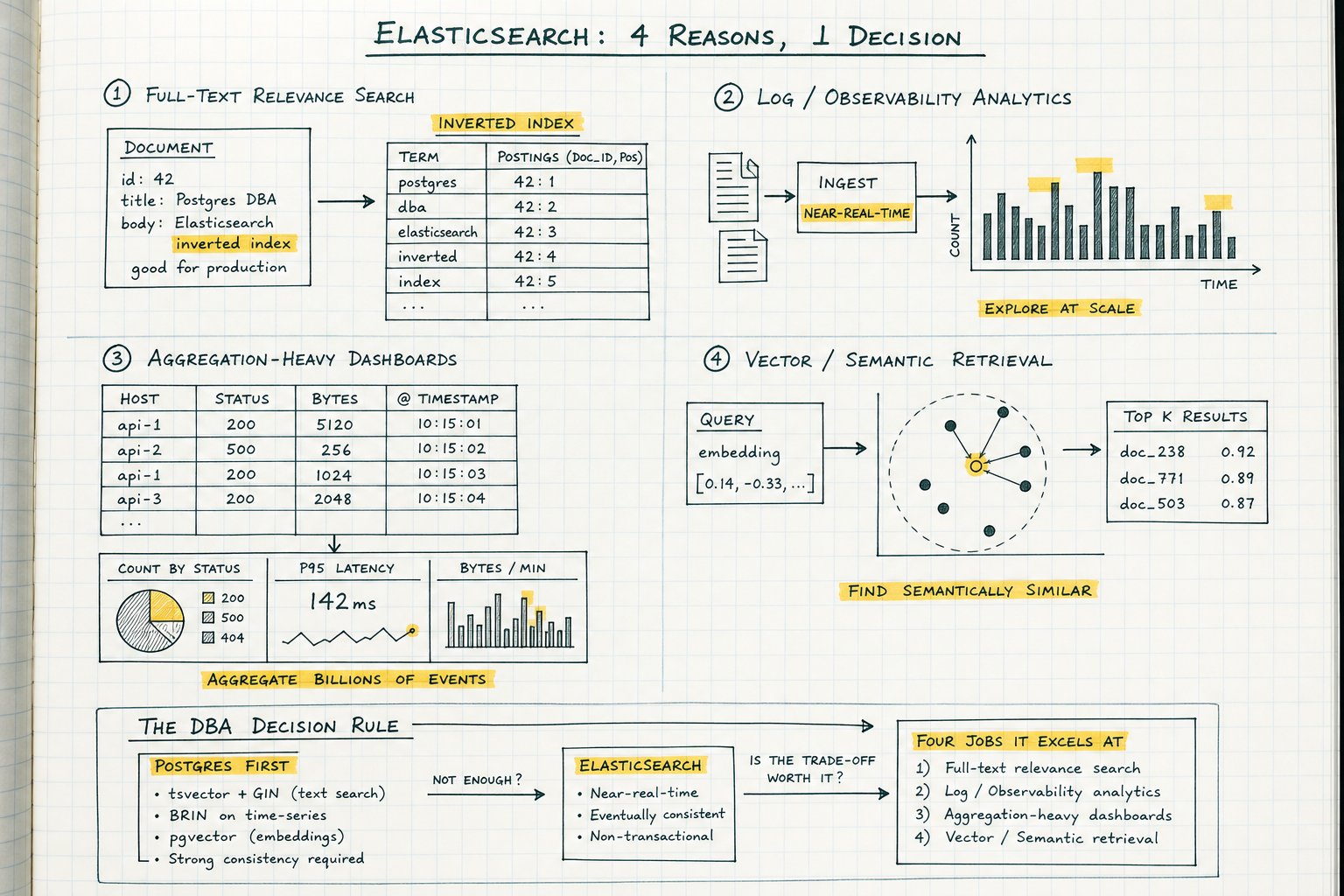
Knowing which job is which saves you a second datastore, a second on-call rotation, and a sync pipeline that will page you at 3am.
What is Elasticsearch, in one paragraph a DBA will recognise?
Structurally, Elasticsearch is a distributed document store wrapped around Apache Lucene. Every shard is a self-contained Lucene index made of immutable segments. When you update a document, nothing is updated in place — the old one is marked deleted, a new one is written, and background merging eventually rewrites segments to reclaim the space. Inside those segments live two structures that matter: an inverted index (term → list of documents containing it), which is what makes text matching fast, and doc_values, a columnar on-disk layout written at index time, which is what makes sorting and aggregations fast. Durability comes from a per-shard translog that is fsynced on every request by default. Visibility comes from a separate refresh cycle, which is why Elasticsearch is described as near real-time rather than real-time.
Hold onto that architecture. Every use case below, and every limitation, falls out of it.
Elasticsearch use case 1: full-text search with relevance ranking
The obvious one. What you actually buy is a specific pipeline: analyzers that tokenize and normalize text, stemming, stopword handling, synonym expansion, edit-distance fuzzy matching, per-field boosting, highlighting, and BM25 scoring. BM25 has been the default similarity since Elasticsearch 5.0, replacing the older TF/IDF default.
Postgres covers a real chunk of this. tsvector/tsquery with a GIN index gives you stemming through dictionaries, ts_rank and ts_rank_cd for ranking, prefix matching, and phrase search. pg_trgm adds trigram similarity for fuzzy matching and can accelerate LIKE/ILIKE patterns with a GIN or GiST index. Since Postgres 12 you can materialize the tsvector in a generated column instead of maintaining a trigger, which removed most of the ugliness from the old pattern.
Here is the same product search both ways. Postgres:
ALTER TABLE products ADD COLUMN search_doc tsvector
  GENERATED ALWAYS AS (
    setweight(to_tsvector('english', coalesce(name,'')), 'A') ||
    setweight(to_tsvector('english', coalesce(brand,'')), 'B') ||
    setweight(to_tsvector('english', coalesce(description,'')), 'C')
  ) STORED;

CREATE INDEX products_search_idx ON products USING GIN (search_doc);

SELECT id, name, ts_rank_cd(search_doc, q) AS score
FROM products, websearch_to_tsquery('english', 'waterproof hiking boot') q
WHERE search_doc @@ q
  AND in_stock
ORDER BY score DESC
LIMIT 20;
Elasticsearch:
{
  "query": {
    "bool": {
      "must": [{
        "multi_match": {
          "query": "waterproof hiking boot",
          "fields": ["name^3", "brand^2", "description"],
          "fuzziness": "AUTO",
          "type": "best_fields"
        }
      }],
      "filter": [{ "term": { "in_stock": true } }]
    }
  },
  "highlight": { "fields": { "name": {}, "description": {} } },
  "aggs": {
    "by_category": { "terms": { "field": "category.keyword", "size": 10 } }
  },
  "size": 20
}
Both return ranked, stemmed, filtered results. The differences are concrete. setweight gives you four weight buckets, A through D; ^3 gives you an arbitrary float per field, and you can change it per query without touching the stored data. Postgres has no built-in equivalent to fuzziness: AUTO inside the full-text match — you bolt on pg_trgm and combine scores yourself. Synonyms in Postgres live in a dictionary file on the server and require a reload to change; in Elasticsearch they can be applied at query time through a search analyzer. Multi-language corpora in Postgres mean a tsvector per language or a per-row regconfig; Elasticsearch handles it with per-field analyzer chains. And the facet counts in that aggs block have no cheap Postgres equivalent when the result set is large.
Postgres loses on relevance-tuning depth. The ranking itself is fine — it’s the knobs that are missing. If your product team is iterating weekly on boosts, synonym lists and analyzer chains, you will feel it. If “match the words, rank sensibly, filter by stock” is the requirement, Postgres handles it and you saved yourself a whole system.
Elasticsearch use case 2: logs, metrics and observability
This is arguably the dominant real-world deployment, and it is where a Postgres shop should stop fighting.
The shape of log data suits Lucene almost perfectly. Writes are append-only. Documents are never updated, so segment immutability costs nothing. The natural partition key is time, and Elasticsearch’s data streams create a rolling series of backing indices automatically. Dynamic mapping means a new field in a log line gets indexed without a migration, though this is also a source of the mapping-drift problems noted below. Kibana sits on top and gives operations people a query box instead of a ticket queue.
Index Lifecycle Management is the part that actually wins the argument. An ILM policy moves an index through hot, warm, cold, frozen and delete phases. Hot nodes take the writes on fast local disk. Warm holds recent-but-not-current data on cheaper hardware. Cold and frozen can be backed by searchable snapshots in object storage, so the data stays queryable while the bytes live in S3 rather than on your SSDs.
A realistic 30-day retention policy for application logs looks roughly like this: roll over the write index at 50GB or 1 day, whichever comes first; move to warm at 3 days with a force-merge and reduced replica count; move to cold at 7 days as a searchable snapshot; move to frozen at 14 days; delete at 30. Queries against the last three days stay fast. Queries against day 25 are slow, and that’s the deal you signed.
Getting the same behaviour in Postgres means declarative partitioning by day, BRIN indexes on the timestamp column, pg_partman for rotation, and a detach-and-archive job. That works, and for modest volumes I have run it happily. It stops working when ingest gets heavy: every log line becomes a row with WAL, MVCC bloat, autovacuum pressure and index maintenance on a table nobody will ever update. Elasticsearch skips all of that because it never pretended to be transactional in the first place.
The rule I use: if you are ingesting logs at a rate where WAL volume from the log table alone materially affects your replication or backup story — tens of thousands of events per second sustained, with retention measured in months — stop optimizing Postgres and go get the ELK stack. It’s not a close call.
Elasticsearch use case 3: aggregations, analytics and dashboards
terms, date_histogram, cardinality, percentiles, nested sub-aggregations — these run off doc_values, the columnar structure, not the inverted index. That is why a facet count over tens of millions of documents returns in the low hundreds of milliseconds when the same query against a normalized Postgres schema is a sequential scan and a hash aggregate.
Be honest about what you get back, though. In a sharded cluster the terms aggregation returns approximate counts, because each shard computes its own top terms independently before they get merged. Elasticsearch tells you so in the response via doc_count_error_upper_bound and sum_other_doc_count — read those fields, they exist for a reason. The cardinality aggregation is approximate too, implemented with HyperLogLog++ and tuned by precision_threshold. There are no SQL-style joins across indices; relationships are handled by denormalisation, nested documents or join fields, each with real cost. There are no multi-document transactions.
The accurate framing: fast approximate slicing over wide denormalised documents. That’s genuinely useful for an operational dashboard and a poor fit for a warehouse. If finance is reconciling numbers off it, you have a problem coming.
Elasticsearch use case 4: vector search and RAG retrieval
Elasticsearch supports dense_vector fields with approximate kNN backed by HNSW graphs, and it can fuse BM25 and vector results with reciprocal rank fusion — which matters in practice because pure vector search alone tends to miss exact keyword and acronym matches that lexical search catches easily. Hybrid retrieval out of the box, with the lexical half already mature, is a genuine advantage.
The counter-argument is strong, though — this is the pgvector vs Elasticsearch question in miniature. pgvector supports both IVFFlat and HNSW (HNSW landed in 0.5.0), and it keeps embeddings in the same row as the source text, inside the same backup, under the same ACID guarantees. Hybrid search is a CTE that unions a tsvector match with a vector distance ordering and re-ranks. When your chunk embeddings and your document metadata are in one place, you can filter by tenant, permission and date in the same query plan without worrying about two systems disagreeing.
My threshold: stay on pgvector until you are past roughly ten million vectors with tight latency requirements, or until you need index build and query throughput that a single Postgres instance cannot supply. Below that, the operational simplicity wins easily. Above it, the dedicated engine starts earning its keep — but by then you probably already run Elasticsearch for something else, which is the real reason to use it.
What is Elasticsearch bad at?
The disqualifiers, plainly:
- No multi-document ACID transactions. None. Per-document operations are atomic and that is the guarantee. A batch of writes across documents can partially succeed.
- No true joins. Denormalise, nest, or use join fields and pay for it — this is a modeling constraint that shapes your whole schema, not a footnote.
- Near real-time, not real-time. Default
index.refresh_intervalis 1 second, so a document you just indexed is not searchable for up to a second. This breaks read-your-own-writes: user saves a record, gets redirected to the search page, does not see it, files a bug. You can force a refresh per request, but doing that on a write-heavy index will wreck your segment count and merge load. Design around it instead — read the canonical row from Postgres after write, not from the index. - Mapping rigidity. You cannot change the type of an existing field in place. Changing it means a new index and a reindex, which on a large index is a planned operation with an alias switch, not a Tuesday afternoon.
- JVM footprint. Set heap to no more than 50% of available RAM (Lucene wants the rest for the page cache) and keep it under roughly 32GB so the JVM can use compressed ordinary object pointers. In practice people cite a safe ceiling somewhere in the 26–30GB range depending on platform. A 64GB node with a 31GB heap is the classic configuration; a 64GB node with a 48GB heap is a classic mistake. This is a Java application with garbage collection pauses to manage, not a lightweight process.
- Eventual consistency during recovery and rebalancing. Shards catch up; queries in the interim may see stale state, and different replicas can briefly disagree before converging.
The summary sentence I want stuck in your head: Elasticsearch is a derived index. It should never be your system of record. If it disappears, you should be able to rebuild it entirely from the source system — treat any cluster you can’t rebuild as a bug in your architecture, not a feature.
Elasticsearch vs Postgres full-text search: the decision rule I actually use
Default position: stay on Postgres. Move only when you hit a named, measured wall. Not a vibe, not “Postgres feels slow” — an actual measured wall. There are four.
Wall 1 — relevance tuning demands. The product team wants per-field boosts, synonyms editable without a deploy, typo tolerance, and A/B testable ranking. ts_rank_cd plus setweight has run out of expressiveness. This is a capability wall, not a performance one, and it is the most legitimate reason of the four.
Wall 2 — log ingest volume. Your log/event table is generating enough WAL to affect replication lag or backup windows, or autovacuum can no longer keep up with the partition churn. Measure it before you claim it.
Wall 3 — aggregation latency. Faceted counts over hundreds of millions of rows are missing your p95 target after you have already tried a covering index, a materialized rollup table and BRIN on the time column. Note the ordering: try the rollup first. A refreshed materialized view has solved this more often than a new cluster has.
Wall 4 — multi-tenant search fan-out. Thousands of tenants each needing isolated ranked search, where per-tenant index or routing genuinely helps and a single Postgres instance can’t give you that isolation without significant sharding work of its own.
If you’re evaluating Postgres full-text search as an Elasticsearch alternative, use this checklist with thresholds rather than vibes:
- Corpus under ~10 million searchable documents, and total tsvector index size fits comfortably in shared buffers plus OS cache.
- Search p95 under your SLO with a GIN index and
websearch_to_tsquery, measured withEXPLAIN (ANALYZE, BUFFERS)on production-shaped data, not on an empty dev box. - Fewer than a handful of relevance-tuning changes per quarter.
- Facet counts either small enough to compute directly or acceptable from a rollup refreshed every few minutes.
- Fewer than roughly 10 million vectors, if RAG is in play.
- No dedicated infrastructure team. This one matters more than the rest combined. A two-person backend team running a three-node Elasticsearch cluster part-time is a bad trade.
If your Postgres full-text search queries are struggling to hit SLO despite good indexing, it’s worth getting a second opinion on the query plans before reaching for a second datastore — that’s the kind of tuning question I get asked most often through MyDBA.
If you do add it: how the data gets there and stays right
Standing up the engine is an afternoon’s work. The sync is what eats your quarter.
Application dual-write. Write to Postgres, then write to Elasticsearch in the same request handler. It drifts. The second write fails, the process crashes between them, a backfill script writes a row directly. Within a month you will be writing a reconciliation job. If you do this, plan the reconciliation job up front.
Scheduled reindex. A cron job that reads rows changed since a watermark and bulk-indexes them. Simple, debuggable, and fine when a minute or two of staleness is acceptable. Watch out for updates that don’t touch updated_at, and for deletes, which need tombstones or a periodic full sweep. It also puts a periodic read load on your primary that grows with table size.
CDC via logical replication. Debezium or Kafka Connect reads the WAL through a logical replication slot and streams changes out. This is the correct answer at scale and it comes with the failure mode that will actually page you: a replication slot holds WAL on the primary until the consumer confirms it. Stop the consumer — deploy gone wrong, Kafka broker down, a poison message — and pg_wal grows until the primary’s disk fills and the database stops accepting writes. Your search index being stale is an inconvenience. Your primary being down is an outage.
Guard it. Set max_slot_wal_keep_size (Postgres 13+) so a stalled slot gets invalidated rather than killing the primary — yes, that means resyncing the consumer from scratch, and that is the right trade. Alert on pg_replication_slots.wal_status and on the lag in bytes between confirmed_flush_lsn and the current LSN. Alert on disk free with enough headroom to act. And test the recovery: kill the consumer for an hour in staging and see what actually happens.
Common questions, answered short
Is Elasticsearch a database? It stores documents and returns them, so mechanically yes. As a system of record, no. No multi-document transactions, no joins, eventual visibility, and mapping changes that require a reindex. Treat it as a derived index over data that lives somewhere durable and relational.
Is it free, and what is OpenSearch? In January 2021 Elastic moved Elasticsearch from Apache 2.0 to a dual SSPL / Elastic License model starting at 7.11. AWS forked 7.10.2 and created OpenSearch, which continues under Apache 2.0. In August 2024 Elastic added AGPL v3 as an additional licence option alongside SSPL and the Elastic License, which addressed some of the original objections but didn’t reunify the two projects. Pick based on your cloud, your support needs and your legal team’s tolerance, and check the current terms rather than trusting this paragraph.
Does it replace my data warehouse? No. terms counts are approximate in a sharded cluster and cardinality is HyperLogLog++. Fine for a dashboard, wrong for anything that gets reconciled.
Do I need Logstash? Usually not. Elastic Agent and Beats cover most shipping, and ingest pipelines handle a lot of transformation inside the cluster. For CDC-style sync from Postgres, Debezium is more common now than Logstash. Logstash earns its place when you need heavy enrichment or fan-out to multiple sinks.
How much RAM? Heap at 50% of node memory, capped below ~32GB so compressed pointers stay on; the other half goes to the page cache for Lucene. 64GB nodes with ~31GB heaps are a sane default. Then size node count by data volume and shard count, not by wishful thinking.
Can I use it as a cache? Please don’t. It is not designed for key-value point lookups at cache latency and the refresh model makes the semantics wrong. Use Redis.
The short answer
Four jobs: relevance search, log and observability analytics, aggregation dashboards, vector retrieval. One architecture explains all four — Lucene segments, an inverted index for matching, doc_values for slicing, near-real-time visibility instead of transactions.
Two rules. Never make it your source of truth. And never adopt it until you have measured the Postgres path failing against a specific number — the cluster itself is the cheap part; the real cost lives in the sync pipeline and the replication slot that quietly fills your primary’s disk on a Sunday.